Bayesian inference with MCMC

This blog post is an attempt at trying to explain the intuition behind MCMC sampling: specifically, a particular instance of the Metropolis-Hasting algorithm. Critically, we’ll be using TensorFlow-Probability code examples to explain the various concepts.

The Problem

First, let’s import our modules. Note that we will use TensorFlow 2 Beta and we will use the TFP nightly distribution with works fine with TF2.

import numpy as np
import tensorflow as tf
import tensorflow_probability as tfp
tfd = tfp.distributions

import matplotlib.pyplot as plt
import seaborn as sns

tf.random.set_seed(1905)

%matplotlib inline
sns.set(rc={'figure.figsize':(9.3,6.1)})
sns.set_context('paper')
sns.set_style('whitegrid')

print(tf.__version__, tfp.__version__)

2.0.0 0.7.0

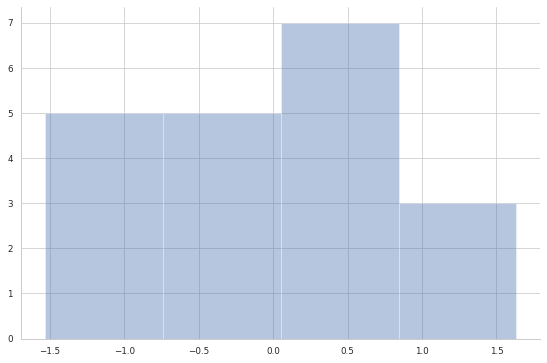
Let’s generate some data: 20 points from a Gaussian distribution centered around zero (the true Data-Generating Process that we want to discover from the 20 samples we can see). Note that in TFP the Gaussian distribution is parametrized by mean and standard deviation, not the variance.

true_dgp = tfd.Normal(loc=0., scale=1.)
observed = true_dgp.sample(20)
sns.distplot(observed, kde=False)
sns.despine();

We have some observations $x$.

Usually (in parametric statistics) we assume a data-generating process, i.e. a model $P(x\mid \theta)$, from which the data we see had been sampled – note that $P$ is used to denote a probability density/mass function. Looking at the data, we come up – somehow – with the idea that a good model for our data is the Gaussian distribution. In other words, we assume that the data are normally distributed.

The model often depends on unknown parameters $\theta$. They can be unknown because they are intrinsecally random or because simply we do not know them. A normal distribution has two parameters: the mean, $\mu$, and the standard deviation, $\sigma$. For simplicity, we assume we know $\sigma=1$ and we want to make inference on $\mu$ only, that is $\theta \equiv \mu$.

From a Bayesian viewpoint, we have to define a prior distribution for this parameter, i.e. $P(\theta)$. Let’s also assume a normal distribution as a prior for $\mu$. Our model can be written as follows (we assumed that the prior is a Gaussian distribution with mean 4 and stardard deviation 2)

In the Bayesian Stat lingo, this way of writing the model derives from the fact that knowing nothing about the joint distribution of the $x$’s’ we can assume exchangeability. By the De Finetti’s Theorem we arrive to the above formulation. Anyway, this goes beyond the scope of this blog post. For more information on Bayesian Analysis look at (the bible) Gelman et al. book.

# prior
mu_0, sigma_0 = 4., 2.
prior = tfd.Normal(mu_0, sigma_0)

# likelihood
mu, sigma = prior.sample(1), 1. # use a sample from the prior as guess for mu
likelihood = tfd.Normal(mu, sigma) 

Digression

Note that actually what I called likelihood, is the likelihood for one specific datapoint – call it $\mathrm{likelihood}i, i=1,\dots,N$. The “proper” likelihood function is (given that we have an _i.i.d. sample) equal to the product of the “per-datapoint” likelihoods

When we consider the loglikelihood, obviously, for an i.i.d. sample, the loglikelihood is the sum of the individual “per-datapoint” likelihoods

Usually, the likelihood is denoted by $\mathcal{L}(\mu; x)$ or $p(x\mid \mu)$.

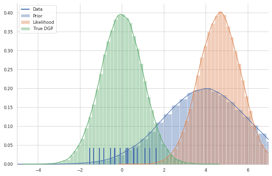
Since we do not know the mean of the Gaussian distribution which generated the data, we use a sample from the prior distribution as a guess for $\mu$ in order to be able to draw it (we need a value), the likelihood has a mean similar to that of the prior distribution.

In the graph below, I plot both the prior and the likelihood, as well as the true data-generating process with the data plotted as a rug

sns.rugplot(observed, linewidth=2, height=0.1)
sns.distplot(prior.sample(10**5))
sns.distplot(likelihood.sample(10**5))
sns.distplot(true_dgp.sample(10**5))
sns.despine()
plt.legend(labels=['Data', 'Prior','Likelihood', 'True DGP'])
plt.xlim(-5, 7);

In the Bayesian framework, inference, i.e. knowing something more about the unknown parameters, is solved by the Bayes formula

The posterior distribution $P(\theta\mid x)$ – that is, what we know about our model parameters $\theta$ after having seen thet data $x$ – is our quantity of interest.

To compute it, we multiply the prior $P(\theta)$ (what we think about $\theta$ before we have seen any data) and the likelihood $P(x\mid \theta)$, dividing by the evidence $P(x)$ (a.k.a. marginal likelihood).

However, let’s take a closer look at this last term: the denominator, $P(x)$. We do not observe it, but we can compute this quantity by integrating over all possible parameter values:

This is the key difficulty with the Bayes formula – while the formula looks pretty enough, for even slightly non-trivial models we cannot compute the posterior in a closed-form way.

NOTE: $P(x)$ is a normalizing constant. Up to this normalizing constant, we know exactly how the unnormalized posterior distribution looks like, i.e.

(where $\propto$ mean “proportional to”). Since we defined both terms on the rhs, we DO know how to sample from the unnormalized posterior distribution

Furthermore, by the product rule – $P(A, B) = P(A\mid B) P(B)$ – we can write

meaning that the unnormalized posterior is proportional to the joint distribution of $x$ and $\theta$.

Back to the example. The prior distribution we defined is convenient because we can actually compute the posterior distribution analytically. That’s because for a normal likelihood with known standard deviation, the normal prior distribution for $\mu$ is conjugate, i.e. our posterior distribution will belong to the same family of distributions of the prior. Therefore, we know that our posterior distribution for $\mu$ is also normal. For a mathematical derivation see here.

Let’s define a function which computes the updates for the parameters of the posterior distribution analytically

def get_param_updates(data, sigma, prior_mu, prior_sigma): #sigma is known
    n = len(data)
    sigma2 = sigma**2
    prior_sigma2 = prior_sigma**2
    x_bar = tf.reduce_mean(data)
    
    post_mu = ((sigma2 * prior_mu) + (n * prior_sigma2 * x_bar)) / ((n * prior_sigma2) + (sigma2))
    post_sigma2 = (sigma2 * prior_sigma2) / ((n * prior_sigma2) + sigma2)
    post_sigma = tf.math.sqrt(post_sigma2)
    
    return post_mu, post_sigma

# posterior
mu_n, sigma_n = get_param_updates(observed,
                                  sigma=1, 
                                  prior_mu=mu_0, 
                                  prior_sigma=sigma_0)
posterior = tfd.Normal(mu_n, sigma_n, name='posterior')

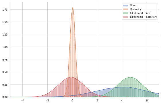
In the graph below, I plot both the prior and the posterior distributions. Furthermore, I plot the likelihood both with mean set to a sample from the prior and a sample from the posterior

sns.distplot(prior.sample(10**5))
sns.distplot(posterior.sample(10**5))
sns.distplot(likelihood.sample(10**5))
sns.distplot(tfd.Normal(posterior.sample(1), 1.).sample(10**5))
sns.despine()
plt.legend(labels=['Prior','Posterior', 'Likelihood (prior)', 'Likelihood (Posterior)'])
plt.xlim(-5, 7);

This shows our quantity of interest (orange): the probability of $\mu$’s values after having seen the data, taking our prior information into account.

The important thing to acknowledge is that, without conjugacy, we would not even be capable of sketching the posterior distribution: we would not know its shape at all. Let’s assume, however, that our prior was not conjugate and we could not solve this by hand – which is often the case.

Approximation methods

When we do not have access to the analytic form of the posterior distribution we can resort to MCMC methods. The basic idea is that we can find strategies to sample from the posterior distribution, even if we cannot “write it down”. These samples are then used to approximate the posterior distribution. One simple strategy to get samples from the posterior distribution is the Rejection Sampling algorithm.

Rejection Sampling

The basic idea of rejection sampling is to sample from an instrumental distribution and reject samples that are “unlikely” under the target distribution. Here we consider a very specific instance of rejection sampling: the Naive Rejection Sampling.

Suppose that you can sample from a joint distribution $P(X, \theta)$ (where $X$ is random as well) – we have seen that we can sample from it since using the product rule we get $P(X, \theta) = P(X\mid \theta) P(\theta)$, which are both defined by us, so we know how to sample from them!

We are interested in sampling $\theta$ from the conditional distribution $P(\theta\mid X = x)$, for some fixed values of $x$ – i.e. the observed data.

The Naive Rejection Sampling algorithm works as follows:

1. Sample $\theta$ from the prior $P(\theta)$ and $X$ from the likelihood $P(X\mid \theta)$

2. If $X = x$ (the observed data) , accept $\theta$ as a sample from the posterior $P(\theta\mid X = x)$ , otherwise return to (1) and repeat

Each time you return to step 1, the samples of $\theta$ are independent from the previous ones.

Pros: step 1 is often practical because both the prior and the likelihood are often easy-to-sample distributions. Cons: the clear shortcoming is that step 2 can be very unlikely and thus we will very rarely (if ever) accept the candidate sample $\theta$.

This simple implementation of rejection sampling is enough to provide some intuition and motivates the use of more sophisticated and robust sampling algorithms based on Markov chains.

MCMC: The Random-Walk Metropolis-Hasting algorithm

There is a large family of algorithms that perform MCMC. Most of these algorithms can be expressed at a high level as follows:

1. Start at current position (i.e. a value for $\theta$, say $\theta^{(1)}$)

2. Propose moving to a new position (say, $\theta^\star$)

3. Accept/Reject the new position based on the position’s adherence to the data and prior distributions

4. • If you accept: Move to the new position (i.e. $\theta^{(2)}=\theta^\star$) and return to Step 1
   • Else: Do not move to new position. Return to Step 1.
5. After a large number of iterations, return all accepted positions.

Based on how you implement the above steps you get the various MCMC algorithm. Here we will review the Random-Walk Metropolis-Hasting algorithm.

As we have seen, the main drawback of the rejection sampling is that it is not efficient – it is unlikely to get exactly $X = x$, especially when it is high-dimensional.

One way around this problem is to allow for “local updates”, i.e. let the proposed value depend on the last accepted value (here is the part where Markov Chains enter the scene).

This makes it easier to come up with a suitable (conditional) proposal, however at the price of yielding a Markov chain, instead of a sequence of independent realizations – putting it simply, a sequence of random variables is a Markov Chain if the future state only depends on the present state.

At first, you find a starting position (can be randomly chosen), lets fix it arbitrarily to

mu_current = 2.

The critical point is how you propose the new position (that’s the Markov part). You can be very naive or very sophisticated about how you come up with that proposal. The RW-MH algorithm is very naive and just takes a sample from a Gaussian distribution (or whatever simmetric distribution you like) centered on the current value with a certain standard deviation, usually called proposal width that will determine how far you propose jumps. In other words, the RW-MH proposes a new $\theta^\star$ according to

where $g$ may be any simmetric distribution. Usually, $g = \mathcal{N}(0, \tau)$, so that the proposed new value, $\theta^\star$, is simply a draw from $\mathcal{N}(\theta_{s}, \tau)$.

proposal_width = 1.
mu_proposal = tfd.Normal(mu_current, proposal_width).sample()

Next, you evaluate whether that’s a good place to jump to or not. To evaluate if it is good, you compute the ratio

Here is the trick: the normalizing constants cancel out. We only have to compute the numerator of the Bayes’ formula, that is the product of likelihood and prior. We have seen that it is the same as computing the joint probability distribution – usually, we compute the log joint probability in practise – of the data and the parameter values. TFP performs probabilistic inference by evaluating the model parameters using a joint_log_prob function that the user as to provide (which we define below).

Then,

• If $\rho\geq1$, set $\theta^{s+1}=\theta^\star$

• If $\rho<1$, set $\theta_{s+1}=\theta^\star$ with probability $\rho$, otherwise set $\theta_{s+1}=\theta_s$ (this is where we use the standard uniform distribution – in practice you draw a sample $u \sim \mathrm{Unif}(0,1)$ and check if $\rho > u$; if it is you accept the proposal)

To sum up, we accept a proposed move to $\theta^\star$ whenever the density of the (unnormalzied) joint distribution evaluated at $\theta^\star$ is larger than the value of the unnormalized joint distribution evaluated at $\theta_s$ – so $\theta$ will more often be found in places where the unnormalized joint distribution is denser.

If this was all we accepted, $\theta$ would get stuck at a local mode of the target distribution, so we also accept occasional moves to lower density regions.

NOTE: The model we define enters the inference scheme only when we evaluate the proposal. In other words, the model we define is important made explicit in the definition of the joint_log_prob function, that is

joint_log_prob = model definition

Let’s now define the joint log probability of the normal model above.

# definition of the joint_log_prob to evaluate samples
def joint_log_prob(data, proposal):
    prior = tfd.Normal(mu_0, sigma_0, name='prior')
    likelihood = tfd.Normal(proposal, sigma, name='likelihood')
  
    return prior.log_prob(proposal) + tf.reduce_mean(likelihood.log_prob(data))

Let’s evaluate the proposal above, i.e. mu_proposal

# compute acceptance ratio
p_accept = joint_log_prob(observed, mu_proposal) / joint_log_prob(observed, mu_current)
print('Acceptance probability:', p_accept.numpy())

Acceptance probability: 1.0373609

It is more than 1, therefore we accept directly. Imagine that p_accept was $0.8$, then we would have drawn a sample from the uniform distribution and check the following

if p_accept > tfd.Uniform().sample():
    mu_current = mu_proposal
    print('Proposal accepted')
else:
    print('Proposal not accepted')

Proposal accepted

At this point we would restart the process again.

TFP implementation

In TFP the algorithm is implemented as follows.

First we define how the step should be taken, i.e. how the proposal should be made. Since we are implementing the RW-MH algorithm we use the function tfp.mcmc.RandomWalkMetropolis. It takes as argument the unnormalized join distribution that it will use to compute the acceptance ratio. The only thing we have to remenber is that we have to “lock the data” or “define a closure” over our joint_log_prob function. In other words, fix the data input of the function joint_log_prob

# define a closure on joint_log_prob
def unnormalized_log_posterior(proposal):
    return joint_log_prob(data=observed, proposal=proposal)

Now we can pass the unnormalized_log_posterior as the argument of the function which implements the step

rwm = tfp.mcmc.RandomWalkMetropolis(
    target_log_prob_fn=unnormalized_log_posterior
)

Secondly, we have to define the initial state of the chain, say $\theta_0$. We choose this arbitrarily.

initial_state = tf.constant(0., name='initial_state')

Finally, we can sample the chain with the function tf.mcmc.sample_chain, which returns the samples (named trace usign the usual stat lingo) and some additional information regarding the procedure implemented (kernel_results)

trace, kernel_results = tfp.mcmc.sample_chain(
    num_results=10**5,
    num_burnin_steps=5000,
    current_state=initial_state,
    num_steps_between_results=1,
    kernel=rwm, 
    parallel_iterations=1
)

However, to take full advantage of TF, we will enclose this sampling process into a function and we will decorate it with tf.function

@tf.function
def run_chain():
    samples, kernel_results = tfp.mcmc.sample_chain(
        num_results=10**5,
        num_burnin_steps=5000,
        current_state=initial_state,
        kernel=rwm,
        parallel_iterations=1,
        trace_fn=lambda _, pkr: pkr)
    
    return samples, kernel_results

Note: To print the code generated by tf.function on fn, use

 tf.autograph.to_code(fn.python_function)

trace, kernel_results = run_chain()
plt.plot(trace);

sns.distplot(prior.sample(10**5))
sns.distplot(posterior.sample(10**5))
sns.distplot(trace)
sns.despine()
plt.legend(labels=['Prior','Analytic Posterior', 'MCMC Posterior'])
plt.xlim(-5, 7);

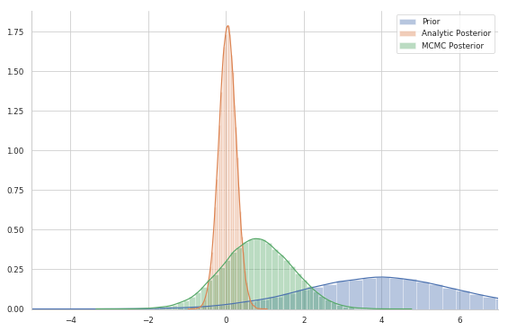
As you can see, even after $10^5$ samples, the MCMC posterior is not even close to the true posterior. That’s normal since the RW-MH algorithm is not very efficient: it is not a great sampler for this kind of problems. You might need a crazy number of samples before it gets close to the true posterior.

On the other hand, other frameworks like PyMC uses the NUTS sampler – a kind of adaptive Hamiltonian Monte Carlo method. TFP supports HMC (tfp.mcmc.HamiltonianMonteCarlo), but still you might have to tune the step size and leapfrog steps parameters (this is the thing that NUTS does adaptively for you). That alone should get you closer to consistent results.

For more material on this subject consult Thomas Wiecki’s Blog, Bayesian Methods for Hacker book, Duke University STAT course page, and this lecture notes for a technical review of Monte Carlo Methods. The material covered here was inspired by Thomas Wiecki’s blogpost.

In a future blogpost I will discuss in more detail both the TFP implemetation of MCMC methods and the diagnostics of the MCMC procedure.

Bonus: PyMC3 implementation with NUTS

Without going into the detail of the procedure (left as a future blogpost), below I implement the same procedure, but using pymc3 and its default sampler (NUTS)

import pymc3 as pm

with pm.Model() as model:
  mu = pm.Normal('mu', mu=4., sigma=2.)
  x = pm.Normal('observed', mu=mu, sigma=1., observed=observed)
  trace_pm = pm.sample(10000, tune=500, chains=1)

100% |██████████|  10500/10500 [00:05<00:00, 1971.43it/s]

sns.distplot(posterior.sample(10**5))
sns.distplot(trace_pm['mu'])
sns.distplot(trace)
plt.legend(labels=['Analytic Posterior', 'PyMC Posterior', 'TFP Posterior']);

As you might notice, just after $10^4$ samples, the NUTS is able to retrieve the true posterior (they are in fact indistinguishable).